Page History
...
Considering geospatial factors is becoming increasingly prominent in many statistical domains. Given the nature of transport statistics, being able to identify and visualize the movement of goods and people between different sub-national regions is of particular relevance. This page shares a few examples of existing sources for these data at the international level, principally UNECE censuses and Eurostat regional data, and techniques for visualising them. Transport statisticians who wish to collaborate on this at future meetings of the Working Party on Transport Statistics are invited contact the secretariat.
Background and Resources
...
The secretariat has tried to map these straight lines onto the real network. As no Shapefiles currently exist of the AGC network, the European TEN-T core network was used instead. The preliminary results for goods trains can be explored at https://rpubs.com/BlackburnStat/ERAIL_Goods. (See below for further details.
Eurostat Regional (NUTS 2 and NUTS 3) Data for Road, Rail and Inland Water
...
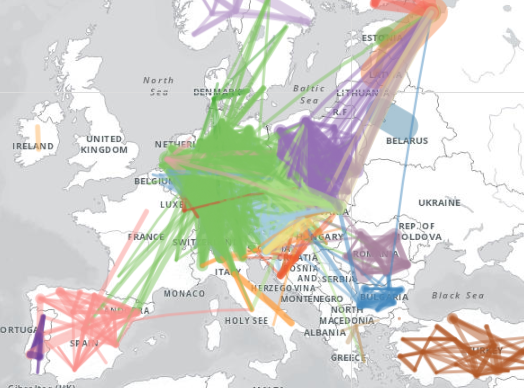
As mentioned, just the international journeys can be filtered out if desired. The following figure shows all international rail passenger journeys 9from (shown in the dataset) greater than 50,000 passengers a year. This map shows, for example, the prominence of Paris and Vienna as international rail hubs, and also shows that the top five origin-destinatino destination combinations are:
- Malmo-Copenhagen
- FlokestoneFolkestone-Calais (Eurotunnel)
- London-Paris (Eurostar)
- Stuttgart-Geneva&Lausanne
- Paris-Brussels
...
These data can be similarly processed and be used to create a map of rail freight. This map can be browsed at https://rpubs.com/BlackburnStat/690015.
Inland Water Freight
The iww_go_atygofl dataset contains similar data to the rail freight numbers, but has the added benefit of breaking data down by type of good according to the NST2007 classification.
...
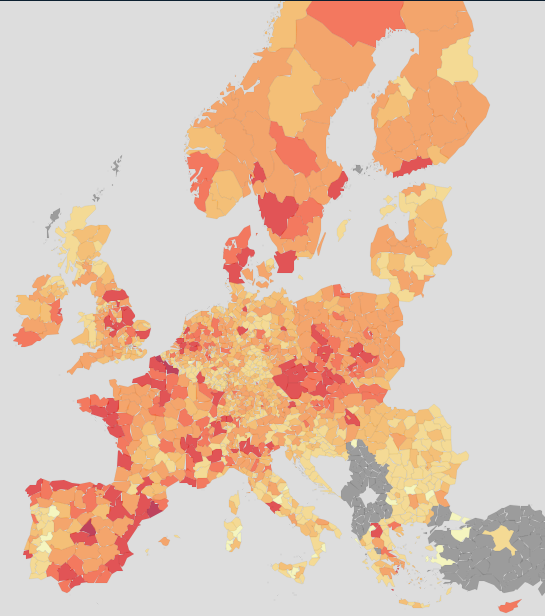
In contrast to the rail and inland water data, there are no published origin-destination linked data for road freight, as this would breach statistical confidentiality. Two similar datasets give freight performance by either region of loading (road_go_ta_rl) and region of unloading (road_go_ta_ru), respectively.
...
Data availability is essentially complete for EU and EFTA countries. The below map shows region of loading, coloured by loaded quantity. The interpretation of the visualisation is somewhat complex; while on the one hand the darker areas represent areas with more goods loaded and therefore therefore more commerce and industry, there are also highly industrialised areas (e.g. along the Rhine) with low values due to the favorising of inland water transport and rail. The differing sizes of regions A further challenge is that different regions have different sizes, which also distorts the picturevisualisation.
Other road data
Unfortunately no regional road passenger data are currently disseminated.
...
In the origin-destination visualisations above, connecting lines are based on the centroids of the origin and destination regions. At the aggregate level this provides a reasonable level of accuracy for the visualisation, but it this runs into problems when there are multiple lines with similar origins and destinations that cannot easily be conceptualised. It would obviously be better if the route fitted the real pattern of the network instead. How can this be done?
...
The problem, however, is that a Shapefile is a collection of line features, which is not a network in the mathematical sense of a graph with nodes (or vertices) and edges (or links): line features do not know what they are connected to, nut network elements do. In order to transform the graphic into a fully-fledged network, the sf library can be used (described clearly in this step-by-step R-spatial blogpost.) This method has the advantage of being able to transfer data from a geospatial data structure to a simple data frame structure and back again, in a single command, which makes manipulating the output very straightforward.
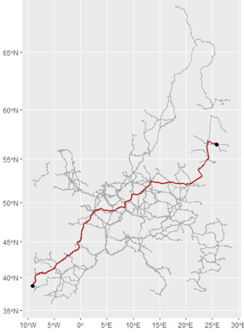
Running the sf code transformation on the AGC (rail) network works well. The below left graph shows the "betweenness" of each node; thus the yellow and orange nodes are the ones most connected to the rest of the network. In order to test to see if the result is behaving like a network, a sample long-distance journey between Portugal and Latvia is simulated, and the network does indeed seem to find the shortest path (which of course may not always follow the most likely path, not considering line speed, traffic levels etc).
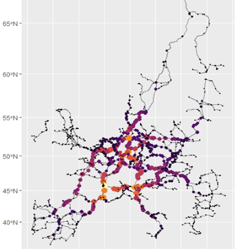
The same is done for the AGN (inland water) network below, between Rotterdam and Poland.
...
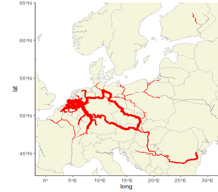
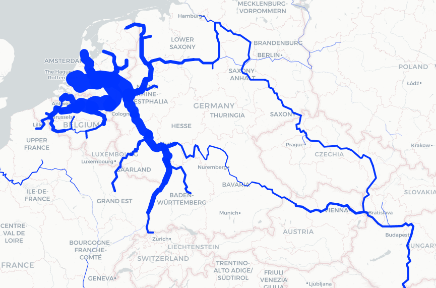
The final step in the process was to collate all individual paths. For this the overline function of the StPlanR package in R can be used. This gives the following result for the inland waterway network in 2019. The code for this can be found at https://github.com/blackburnstat/Mapping_IWW_tonnage.
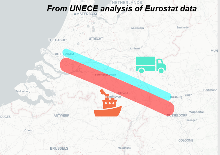
Modal Split Analysis for Specific Corridors
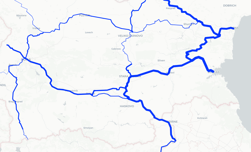
Combining the data for multiple modes would be a logical next step in this analysis. This would allow modal split calculations to be done for specific corridors (like in the picture below), allowing identification of modal shifting opportunities to less polluting and safer modes for both passenger and freight transport.
Resources
Much of the geospatial analysis needed to produce the route maps above uses the sfnetworks and stPlanR packages in R. The transport chapter of Geocomputation with R is a good place to start work on this topic.
Overview
Content Tools
Apps