Introduction
This Page is a Work in Progress
Considering geospatial factors is becoming increasingly prominent in many statistical domains. Given the nature of transport statistics, being able to identify and visualize the movement of goods and people between different sub-national regions is of particular relevance. This page shares a few examples of existing sources for these data at the international level, principally UNECE censuses and Eurostat regional data, and techniques for visualising them. Transport statisticians who wish to collaborate on this at future meetings of the Working Party on Transport Statistics are invited contact the secretariat.
Background and Resources
E-Roads of the AGR Network – E-Roads are defined in the 1975 European Agreement on Main International Traffic Arteries (AGR). https://unece.org/DAM/trans/doc/2016/sc1/ECE-TRANS-SC1-2016-03-Rev1e.pdf.
E-Rail lines of the AGC Network – E-Rail lines are defined in the European Agreement on Main International Railway Lines of 1985 (AGC), https://unece.org/DAM/trans/doc/2019/sc2/ECE-TRANS-63-Rev.4e.pdf.
E-Inland Waterways of the AGN Network –
NUTS classification – regions are classified according to the Nomenclature of Units for Territorial Statistics (NUTS). The NUTS serves as a reference for the collection, development and harmonisation of EU regional statistics and for socio-economic analyses of the regions (more information is available on Eurostat's website: http://ec.europa.eu/eurostat/web/nuts/overview). Several Eurostat datasets are based on movements between NUTS2 regions.
Software used
In order to allow reproducibility, open-sources statistical software was used for all analyses, namely R (utilising RStudio).
The script files used for production of any maps below are either linked to below or are available on request. The scripts are written in a way that should allow any user to run them and recreate the same maps. If a user is new to R, then each library referenced at the start of each script will need to be installed (only once). E.g.
install.Packages("tidyverse").UNECE E-Road and E-Rail Censuses
E-Road Census
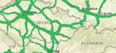
The UNECE E-Road Census collects traffic volumes on principal road arteries of international importance. Data are only collected every five years. Data for 2020, 2015 2010 and 2005 can be explored here https://www.unece.org/trans/main/wp6/e-roads_maps.html. Unfortunately only a limited number of UNECE countries provide data in a geospatial format that allows this visualization. Some countries do have traffic counts at specific points and the secretariat is exploring ways to help countries produce similar outputs with these traffic counts as inputs.
E-Rail Census
The UNECE E-Rail census collects data on principal rail routes, as defined by the AGC, in a similar fashion to the E-Road census. Rail traffic has the advantage of the split between passenger and freight trains is normally easy to make, therefore traffic for either the movement of people or goods can be visualised separately.
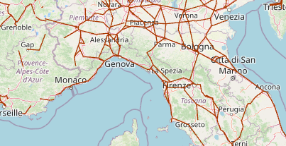
Due to the way the data are collected, Shapefiles that model the real shape of the network are typically not available, but origin-destination lines can be created. Depending on how well segmented the data are, these can often fit the realities of the country's geography quite well. Explore the data here https://www.unece.org/trans/areas-of-work/transport-statistics/statistics-and-data-online/e-rail-census/traffic-census-map.html.
Eurostat Regional (NUTS 2 and NUTS 3) Data for Road, Rail and Inland Water
In addition to the census data collected directly by UNECE, Eurostat collects many different regional datasets that can be visualised, some of which are on an annual basis. While the UNECE censuses collect traffic volumes, i.e. number of vehicles per day, the Eurostat data focus on transport measurement, that is passenger numbers and passenger-km, tonnes and tonne-km. Examples of possible visualisations are
Rail Passengers
There is only one Eurostat passenger rail dataset that contains data below the national level. The "tran_r_rapa" set covers both national and international railway passengers transported by loading and unloading NUTS 2 region.
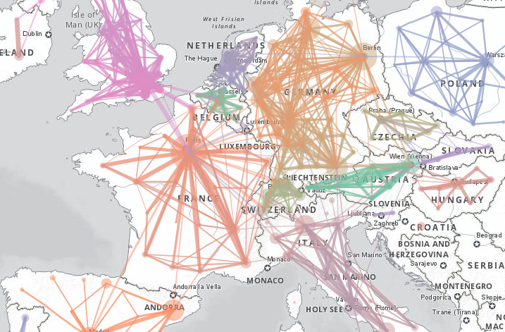
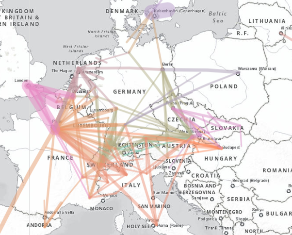
There are national-level international rail journey datasets available, but this regional dataset has the benefit of collecting information from both the origin and destination country, which means that less data are unavailable due to confidentiality (as long as one country publishes the figures, then they are visible). Data can thus be visualised, but given the large number of connections with very small numbers of passengers, some filtering makes sense. The picture below shows a map with all flows greater than 100,000 passengers a year. The map shows, for example, interesting difference sin traffic between France, where most flows connect with Paris, and Germany, where the flows are much more spread out between multiple large cities.
This map can be browsed in an interactive format at https://rpubs.com/BlackburnStat/689627.
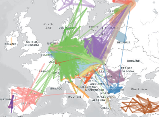
As mentioned, just the international journeys can be filtered out if desired. The following figure shows all international rail passenger journeys 9from the dataset) greater than 50,000 passengers a year. This map shows, for example, the prominence of Paris and Vienna as international rail hubs, and also shows that the top five origin-destinatino combinations are:
- Malmo-Copenhagen
- Flokestone-Calais (Eurotunnel)
- London-Paris (Eurostar)
- Stuttgart-Geneva&Lausanne
- Paris-Brussels
This map can be viewed interactively at https://rpubs.com/BlackburnStat/689644.
Rail Goods
On the freight side, a similar dataset is collected between origin and destination NUTS2 regions, named tran_r_rago. Again, this dataset is asked for only every five years.
These data can be similarly processed and be used to create a map of rail freight. This map can be browsed at https://rpubs.com/BlackburnStat/690015
Inland Water Freight
The iww_go_atygofl dataset contains similar data to the rail freight numbers, but has the added benefit of breaking data down by type of good according to the NST2007 classification.
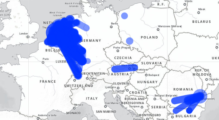
The screenshot below shows all flows above 500,000 tonnes in 2018 (unlike the rail data, the inland water data are collected annually). View this map at https://rpubs.com/BlackburnStat/690029.
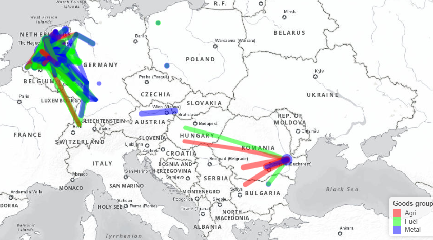
NST2007 has too many categories to easily visualize, but it is possible to combine a few different categories. The above (right) map compares three broad good types: "Agri" contains, agricultural products, forestry products and food; "Fuel" contains primary and secondary fossil fuels; and "Metal" contains primary and secondary metallic products, as well as chemicals. This map is available at https://rpubs.com/BlackburnStat/690030.
(see also Collating multiple journeys below).
Road
Road freight
In contrast to the rail and inland water data, there are no published origin-destination linked data for road freight. Two similar datasets give freight performance by either region of loading (road_go_ta_rl) and region of unloading (road_go_ta_ru), respectively.
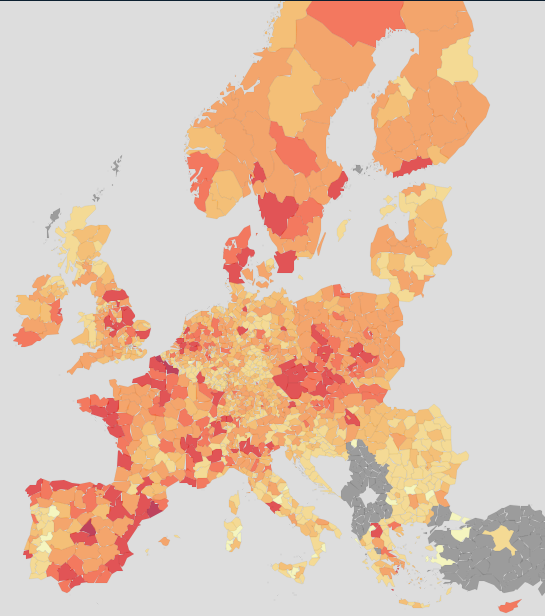
Data availability is essentially complete for EU and EFTA countries. The below map shows region of loading, coloured by loaded quantity. The interpretation of the visualisation is somewhat complex; while on the one hand the darker areas represent areas with more goods loaded and therefore more commerce and industry, there are also highly industrialised areas (e.g. along the Rhine) with low values due to the favorising of inland water transport and rail. The differing sizes of regions also distorts the picture
Other road data
Unfortunately no regional road passenger data are currently disseminated.
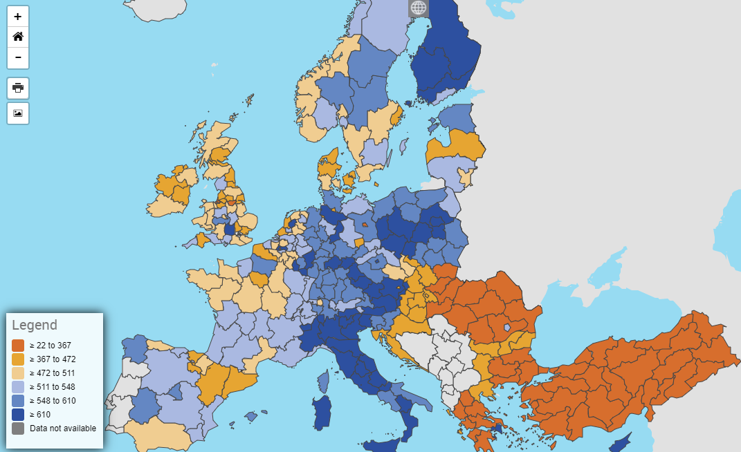
The number of passenger cars per thousand inhabitants is an interesting indicator of how much cars are used in different regions compared to public transport, although it is also related to income as well. These data can be visualised on the Eurostat website directly here https://ec.europa.eu/eurostat/databrowser/view/TRAN_R_VEHST__custom_250445/default/map?lang=en.
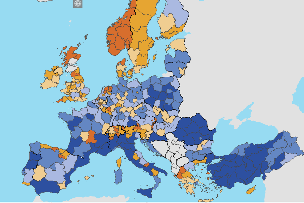
Road accidents per million inhabitants by region can be plotted in a similar way. There is an important disclaimer to note, which is that this will likely overrepresent the road danger in some sparsely populated regions that have principal roads passing through them. The below image is sourced directly from Eurostat's data browser https://ec.europa.eu/eurostat/databrowser/view/tran_r_acci/default/table?lang=en.
Transforming Straight Lines onto the Real Network
In the origin-destination visualisations above, connecting lines are based on the centroids of the origin and destination regions. At the aggregate level this provides a reasonable level of accuracy for the visualisation, but it would obviously be better if the route fitted the real pattern of the network instead. How can this be done?
The first step is to obtain the relevant network Shapefiles. Through its various infrastructure agreements, UNECE has Shapefiles for the AGN (inland waterways) and AGR (road) agreements. Shapefiles for the AGC (railways) agreement are not yet available, but the TEN-T core rail network files are available and this closely agrees with the AGC network.
The problem, however, is that a Shapefile is a collection of line features, which is not a network in the mathematical sense of a graph with nodes (or vertices) and edges (or links): line features do not know what they are connected to, nut network elements do. In order to transform the graphic into a fully-fledged network, the sf library can be used (described clearly in this step-by-step R-spatial blogpost.) This method has the advantage of being able to transfer data from a geospatial data structure to a simple data frame structure and back again, in a single command, which makes manipulating the output very straightforward.
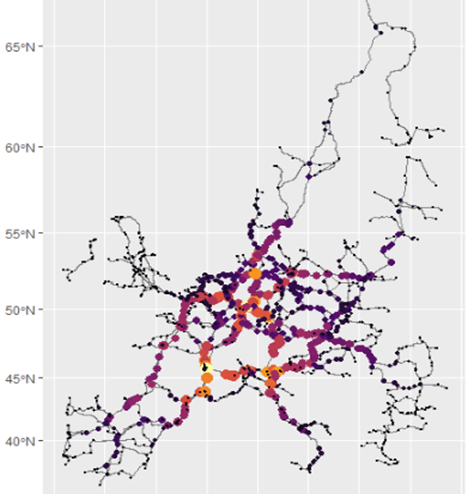
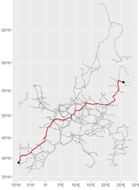
Running the sf code on the AGC network works well. The below left graph shows the "betweenness" of each node; thus the yellow and orange nodes are the ones most connected to the rest of the network. In order to test to see if the result is behaving like a network, a sample long-distance journey between Portugal and Latvia is simulated, and the network does indeed seem to find the shortest path (which of course may not always follow the most likely path).
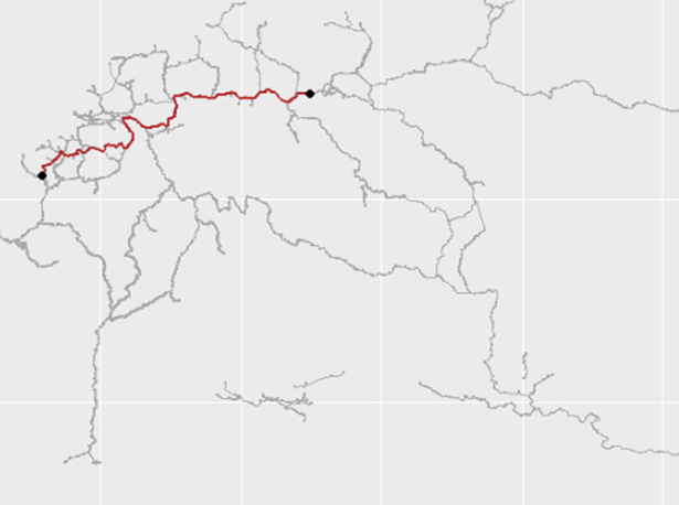
The same is done for the AGN (inland water) network below, between Rotterdam and Poland.
Collating Multiple Journeys
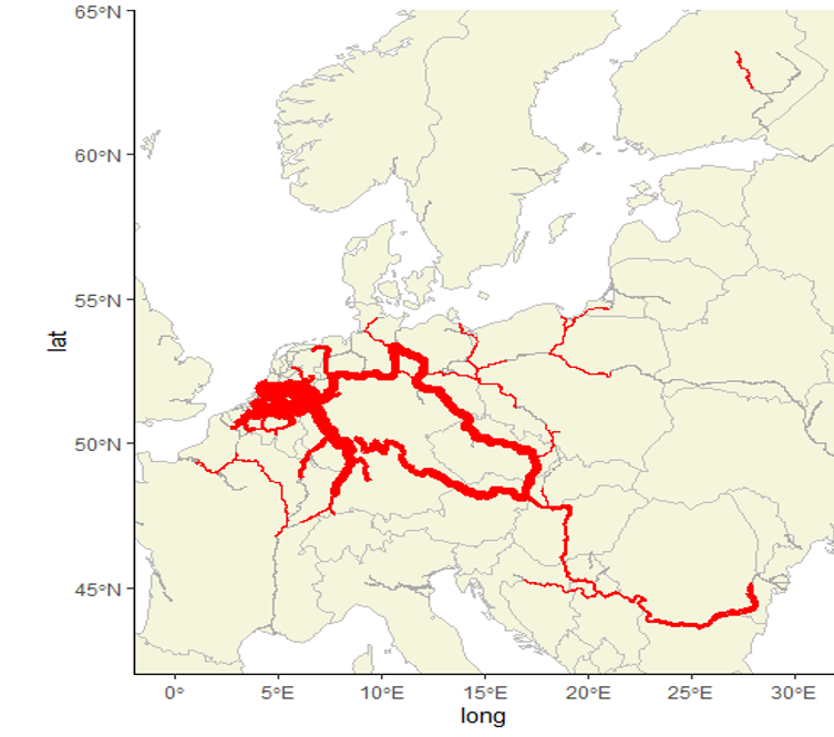
The final step in the process was to collate all individual paths. For this the overline function of the StPlanR package in R can be used. This gives the following result for the inland waterway network in 2019. The code for this can be found at https://github.com/blackburnstat/Mapping_IWW_tonnage.
Modal Split Analysis for Specific Corridors
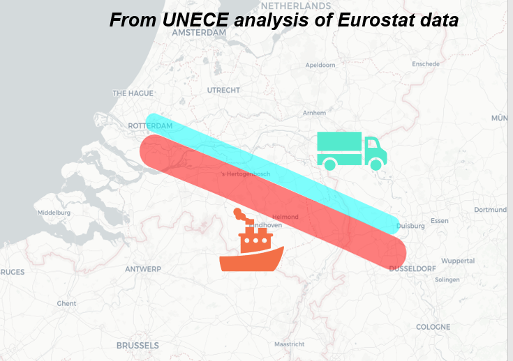
Combining the data for multiple modes would be a logical next step in this analysis. This would allow modal split calculations to be done for specific corridors (like in the picture below), allowing identification of modal shifting opportunities to less polluting and safer modes for both passenger and freight transport.

